Pre-Choice

Order	№	Thème
1	22	Contrôleur PID réglé par réseau de neurones
2	24	Etude et développement d’une solution de commande programmable décentralisée de l’unité de tri de pièces sous environnement Factory IO
3	34	Commande intelligente d’un accélérateur d’un véhicule électrique
4	16	Conception et réalisation d’un système intelligent pour modéliser les machines électriques

Choice

15/02/2026

Thème №22: Contrôleur PID réglé par réseau de neurones

Encadrante: Mme Amoura

Description: Le choix d’une commande s’avère de plus en plus compliqué au regard du nombre important de contrôleurs développés et des différents outils qui facilitent leurs utilisations. Ce choix dépend forcement de la complexité du système à contrôler, des informations disponibles sur le procédé et des différentes perturbations et variations paramétrique affectant le système au cours du temps. La synthèse d’une commande intelligente permet de prendre en compte ces différentes contraintes et également d’élargir le champ d’application à des systèmes plus complexes. En effet, l’utilisation de réseau de neurones permet de mettre à jour les paramètres du PID afin de prendre en compte les différentes variations du système en cours d’utilisation.

Key points

start with a regular PID
PID parameters should be regulated with a neural network
neural network will have one hidden layer
move towards a fractional PID (FOPID)
compare the performance of PID, optimal PID, FOPID, PID with neural network
use matlab r2021

References to check out

Charef, A. (2006). Analogue realisation of fractional-order integrator, differentiator and fractional PID controller. IET Control Theory & Applications, 153(6), 714–722.
Monje, C. A., Chen, Y., Vinagre, B. M., Xue, D., & Feliu, V. (2010). Fractional-order Systems and Controls : Fundamentals and Applications. Springer.
Valério, D., & Sá da Costa, J. (2013). An Introduction to Fractional Control. IET
Monje, C. A., Chen, Y., Vinagre, B. M., Xue, D., & Feliu, V. (2010). Fractional-order Systems and Controls : Fundamentals and Applications. Springer.
Zhao, C., Xue, D., & Chen, Y. Q. (2005). A Fractional Order PID Tuning Algorithmfor a Class of Fractional Order Plants. In International Conference on Mechatronics andAutomation (pp. 216-221). Niagara, Canada.
Liu, L., Wang, Z., & Zhang, H. (2017). A multi-objective optimization method for fractional order PID controller based on robustness and performance indices. ISA Transactions, 72,256–267.
Deep Learning, Ian Goodfellow, Yoshua Bengio & Aaron Courville
PID Tuning with Neural Networks, Antonio Marino and Filippo Ner
Auto tuned PID and neural network predictive controller for a flow loop pilot plant, Sanjay R. Patil, Sudhir D. Agashe

Previous works & understanding

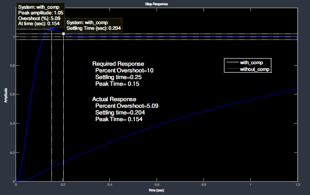
Optimal Fractional Order PID Controller for Speed Control of Electric Vehicle (ACO)

File

Outline

Objective: Control the speed of an EV
Method: Using a Fractional Order PID controller tuned through Ant Colony Optimization (ACO)
Results: Superior performance over a classic PID an an Optimal PID

Breakdown

Section 1 introduces the concept of EVs briefly, lists previous approaches used to regulate EV speed, presents the method studied and outlines the paper’s structure.
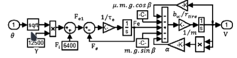
Section 2 models the EV’s dynamics, gives the state space representation, transfer function and the Simulink model.
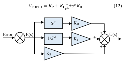
Section 3 briefly explains the PID controller the, introduces the notion of Fractional Order Controllers, lists the four types then focuses on the FOPID. It gives a brief background on fractional Calculus then explains the expression of the differintegral and the fractional differintegral. It ends with the equation and structure of the FOPID.
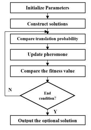
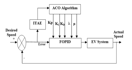
Section 4 gives a detailed explanation of the theory behind Ant Colony Optimization, it then outlines its implementation step by step. It ends with the complete system and controller diagram.
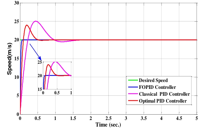
Section 5 shows simulation results in Matlab where the developed FOPID significantly outperforms both a conventional manually tuned PID and an Optimal PID. The system response graphs show the FOPID having no overshoot and an almost negligeable rise time while the other PIDs both have overshoot and a significant settling time.
Section 6 recapitulates the proposed solution, simulation results with digestible. numbers and affirms the benefits of the FOPID. It suggests further improvements like neural networks

Optimal Speed Control of Hybrid Electric Vehicles (LQR)

File

Outline

Objective: Control the speed of an EV
Method: Using an Optimal LQR controller
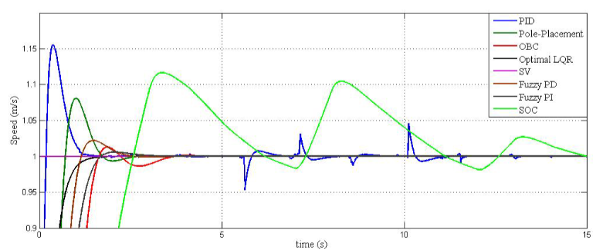
Results: Superior performance over PID, OBC, SOC, and FLC

Breakdown

this project uses the exact same EV representation and numbers

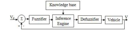
Section 01 introduces the concept of EVs and HEVs and their role in lowering global emissions, it then sets the control problem and looks into previously tried solutions such as Fuzzy Logic Control, LQR Control and other techniques. It ends by setting the goal of finding the superior controller for this application.
Section 2 models the EV’s dynamics, gives the state space representation, transfer function and the Simulink model. It ends by listing the controllers studied below.
Section 03 analyses the open loop stability of the system then deduces the controllability and observability characteristics.
Section 04 gives the transfer function of the PID controller, briefly citing it’s parameters then gives the Simulink model with the PID controller.
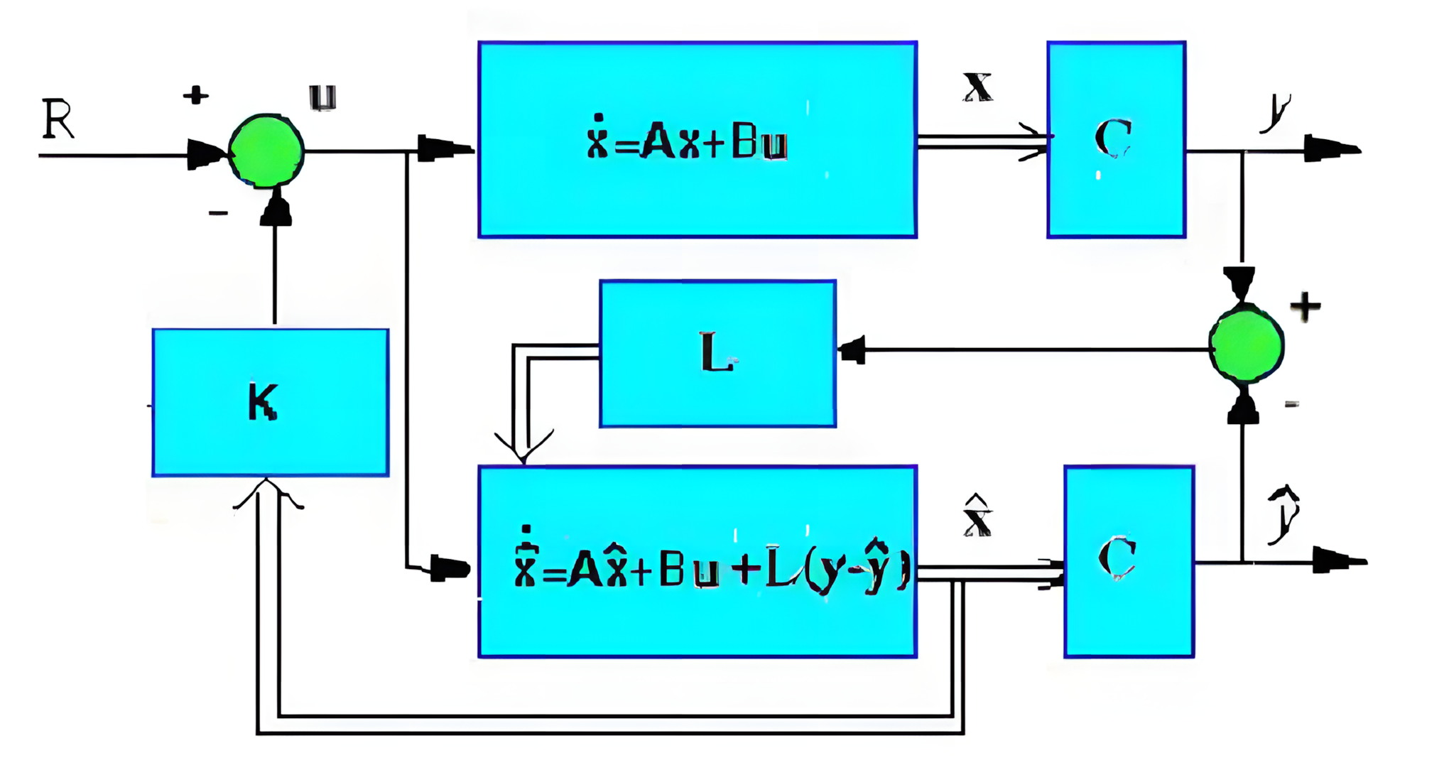
Section 05 is divided into three subsections each explaining a type of state feedback based control pole placement: 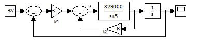$\overset{x}{˙} (t) = A x (t) + B u (t)$ $u (t) = - k x (t)$ $\overset{x}{˙} (t) = (A - B k) x (t)$ $∣ s I - (A - B k) ∣ = 0$ $\sum (s - λ_{i}) = 0$ Observer Based Controller: $D (s) = K (s I - A + B K + L C)^{- 1} L$ Linear Quadratic Optimal Controller $J = \frac{1}{2} x^{T} (t_{f}) S_{x} (t_{f}) + \int_{t_{0}}^{t} \frac{1}{2} [x^{T} Q x + u^{T} R u] d t$ $u (t) = - R^{- 1} (t) B^{T} (t) P (t) x (t)$
Section 06 explains the concept of a Self Organizing Controller (SOC) and gives the Simulink model of an SOC
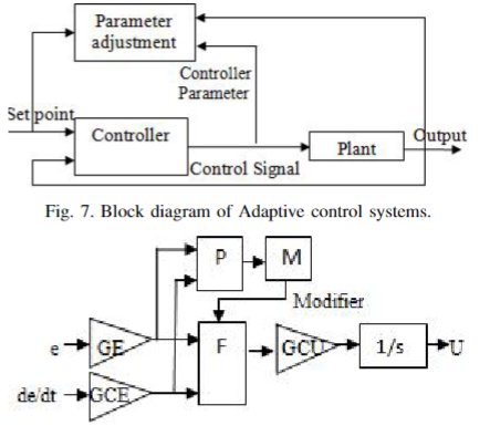
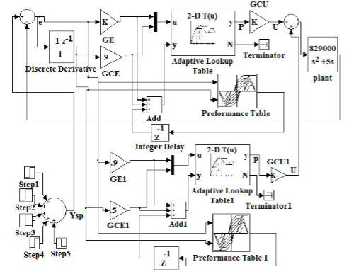
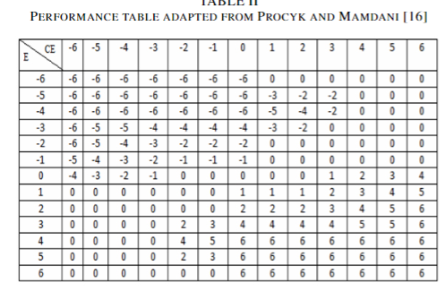
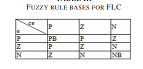
Section 07 explains in details the working of a Fuzzy Logic Controller, it gives the performance table, the fuzzy rule bases, and the block diagram of the system controller by the FLC
Section 08 presents simulation results and compares the open loop uncontrolled response to the closed loop responses with the different studied controllers (PID, Optimal LQR, OBC, SOC, and FLC), the results show that optimal LQR gives better performance index than the other controllers
Section 09 concludes from the comparative analysis that the LQR Optimal controller gives better performance compared to the other studied controllers resulting in better real life performance in terms of current, torque, and battery optimization. It suggests that Optimal LQR may be used in other areas to optimize performances.

Robust adaptive speed control of uncertain hybrid electric vehicle ( $H_{\infty}$ Control)

File

Outline

Objective: Control the speed of an EV
Method: Using $H_{\infty}$ Control
Results: MRAS with RM-1 is better for nonlinear HEV and the $H_{\infty}$ controller is more suitable for linearized HEV

Breakdown

Section 01 introduces the notion of EVs and HEVs emphasizing their importance for the environment, it talks about ETCS and the different ways of controlling throttle position while accounting for the non-linearities and uncertainties. It ends by proposing $H_{\infty}$ Control for a linearized version of the HEV and giving some background and explanations for $H_{\infty}$ Control.
Section 02 starts by explaining the architecture of an HEV and the ETCS, it gives the nonlinear mathematical model and transfer function of the ETCS, then it gives us the model of the nonlinear vehicle and its linearized form, combining the models results in the overall system model.
Section 03 starts with a brief presentation of the PID controller, then explains the implementation of self tuning parameters using fuzzy logic.
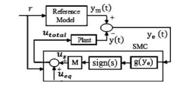
Section 04 starts with a brief explanation of Model Reference Adaptive System (MRAS), it then gives two second order reference models with different parameters. It then explains Sliding Mode Control (SMC) based on Lyapunov’s theory, it then applies SMC to the non linear system model using the linearized one for the observer
Section 05 presents the robust stability analysis of the linearized HEV with parametric uncertainty using the proportional controller (PC) and Kharitonov’s theorem.
- H∞ control is configured with weighting functions, the objective is to design $C (s)$ with the desired tracking performance and robustness. here the mixed-sensitivity approach is used, the goal is to minimize the norm of the sensitivity matrix $∣∣ S (jω) ∣ ∣_{\infty}$ at the output.
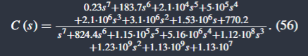
- Kharitonov’s theorem is used to determine the stability margins and conditions of the system, therefore we can find the transfer function with parametric variation.
- Robust stability analysis we consider three cases with different ways of obtaining the gain of $C (s)$ and apply the stability condition on each case.
  - in case 1 the gain is chosen as unitary. we find that the system in unstable.
  - in case 2, we derive the gain from with the root locus technique. we find the system stable with a margin of 0.139.
  - in case 3, we derive the gain using Routh’s order reduction technique. we find the system stable with a margin of 0.32.
- The stability margin obtained from a robust PC, i.e., a PC designed using an H∞ controller, is far better compared to the stability margin obtained from a conventional PC
Section 06 presents the simulation results, it compares the closed loop response of the HEV with various controllers (PI, PID, STF-PID, MRAS, $H_{\infty}$ ) focusing on performance markers such as IAE, ISE, OS, RT and ST.
Section 07 concludes that the MRAS with RM-1 is better for the nonlinear HEV and the $H_{\infty}$ controller is more suitable for linearized HEV

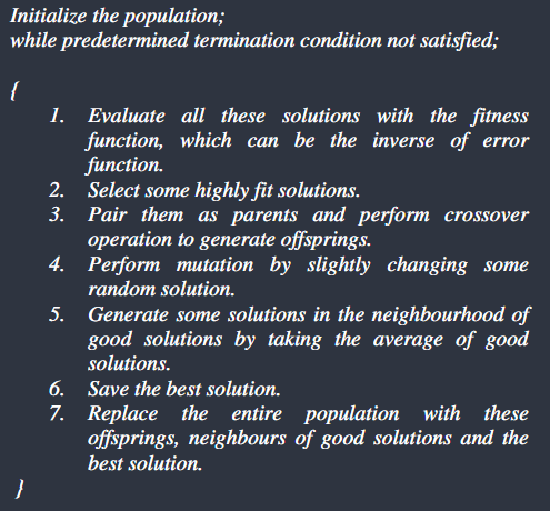
Tuning of PID Controller for DC Servo Motor using Genetic Algorithm

File

Outline

Objective: Control the speed and position of a DC Servo Motor
Method: Using a PID Controller tuned through a Genetic Algorithm
Results: The genetic algorithm based PID tuning provides much better results compared to the conventional methods.

Breakdown

Section 01 introduces DC Servo Motors and the previously used control methods, mainly the conventional PI/PID and suggests improving their implementation by tuning the parameters using a Genetic Algorithm.
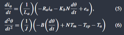
Section 02 gives a mathematical model of a DC Servo Motor
Section 03 explains the PID controller design
Section 04 explains in detail the working of a Genetic Algorithm
Section 05 explains in detail the implementation of a Genetic Algorithm in the case of the PID Controller
Section 06 gives the simulation results, finding that for a wide range of requirements, tuning is done and actual response is found to be better than the required response. Therefore, the gain values of the PID controller are optimized to achieve the desired response.
Section 07 concluded that the genetic algorithm based PID tuning provides much better results compared to the conventional methods. it suggests that the range of requirement can be widened by increasing the range of initial population to achieve a more flexible controller.

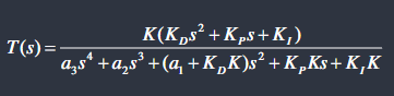
Contrôleur PID d’ordre fractionnaire basé sur la fonction idéale de Bode

File

Outline

Objective:
Method:
Conclusion:

Breakdown

Mémoire Structure

Introduction Générale

Contexte : Importance de la régulation dans l’industrie (plus de 97 % des contrôleurs sont des PID).
Problématique : Limitations du PID classique face aux systèmes non linéaires, incertains ou à paramètres variants (ex: changement de pente pour un véhicule).
Objectif du mémoire : Développer un système d’ajustement intelligent des gains ( $K_{p}, K_{i}, K_{d}$ ) en temps réel via un réseau de neurones pour améliorer la précision, la rapidité et la robustesse.

Chapitre I : État de l’art sur la Commande PID

Le Régulateur PID Classique :
- Principes des actions Proportionnelle, Intégrale et Dérivée.
- Structures possibles (parallèle, série, mixte).
Méthodes de Réglage Conventionnelles :
- Méthodes de Ziegler-Nichols et réglage manuel.
- Limites des approches fixes face aux perturbations.
Introduction au PID d’ordre fractionnaire (FOPID) :
- Généralisation avec les paramètres $λ$ et $μ$ pour plus de flexibilité.

Chapitre II : Fondamentaux des Réseaux de Neurones Artificiels

Architecture d’un Neurone Artificiel :
- Entrées, poids, biais et fonctions d’activation (ReLU, Sigmoïde, Tanh).
Structure du Réseau Multi-couches (MLP) :
- Couches d’entrée, cachées et de sortie.
Apprentissage et Optimisation :
- Algorithme de Rétropropagation de l’erreur (Backpropagation)
- Fonction de coût (MSE) et descente de gradient.

Chapitre III : Modélisation du Système à Commander

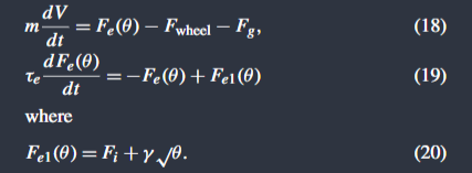
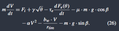
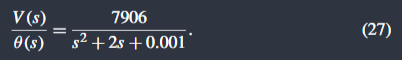
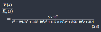
Vitesse d’un Véhicule Électrique (VE) :
- Modélisation des forces (motrice, traînée, gravité).
- Linéarisation autour d’un point de fonctionnement et fonction de transfert.
- Analyse de la commandabilité et de l’observabilité.

Chapitre IV : Conception du PID Auto-réglé par Réseau de Neurones

Architecture du Système de Commande :
- Utilisation du réseau de neurones pour le réglage des gains : le réseau reçoit en entrée l’erreur ( $e$ ) et la variation de l’erreur $d e / d t$ et fournit en sortie les paramètres $K_{p}, K_{i}, K_{d}$ optimaux.
Algorithme d’Ajustement :
- Définition de la topologie (ex: 2 entrées, X neurones cachés, 3 sorties).
- Stratégie d’apprentissage (Supervisé ou Renforcement) pour minimiser un critère comme l’IAE ou l’ITAE.
Extension optionnelle : Intégration du réglage NN sur un contrôleur FOPID pour comparer l’apport de l’intelligence artificielle sur un système déjà robuste.

Chapitre V : Simulation et Analyse des Résultats

Environnement de simulation : MATLAB R2021 / Simulink.
Tests de Performance :
- Réponse indicielle (temps de montée, dépassement, temps d’établissement).
- Évaluation des critères d’erreur (IAE, ITAE, ISE).
Étude Comparative :
- Comparaison entre PID classique, PID optimisé (ex: Algorithme Génétique), FOPID et PID-NN.
Test de Robustesse :
- Réponse du système face à des perturbations externes (ex: échelon de charge ou changement de pente).

Conclusion Générale et Perspectives

Synthèse sur l’efficacité des réseaux de neurones pour l’auto-réglage.
Perspectives : Implémentation sur plateforme embarquée (FPGA/Microcontrôleur) et exploration du Deep Reinforcement Learning.

Neural Networks

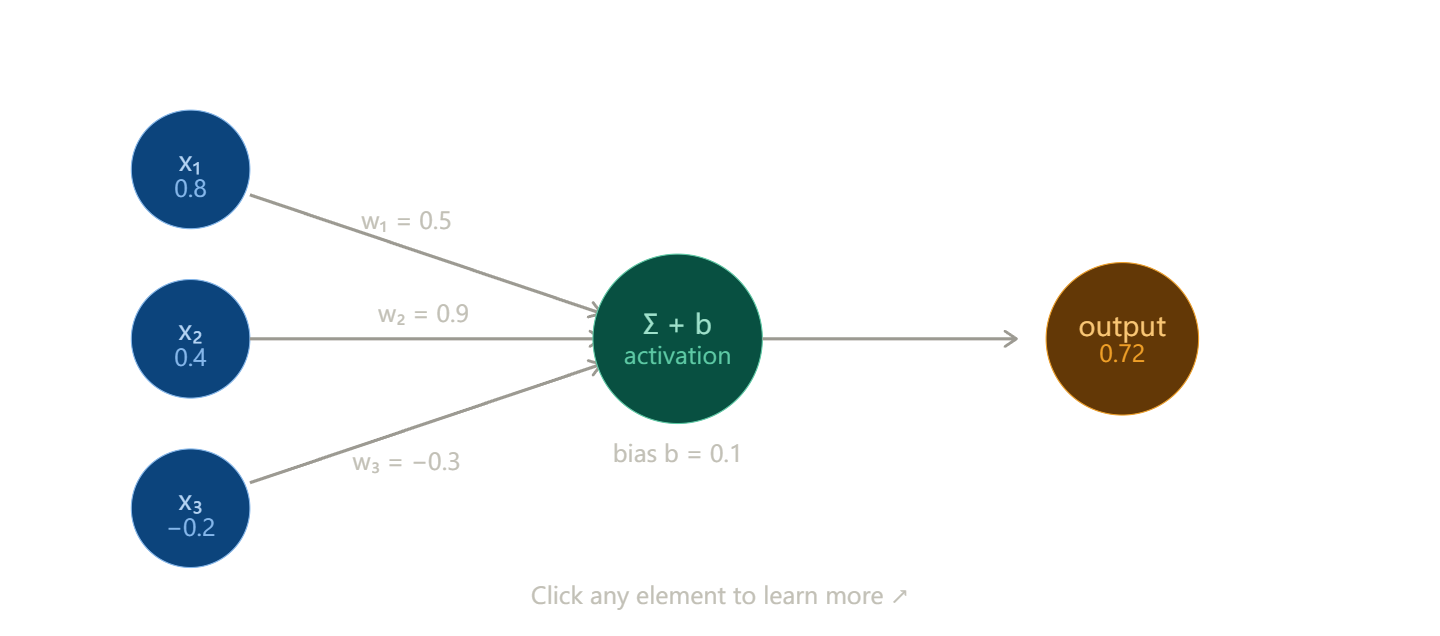
What is a neuron?

The basic unit is a single artificial neuron. It takes several inputs, multiplies each by a weight, sums them up, adds a bias, and passes the result through an activation function that decides whether and how strongly the neuron “fires”.

The formula is simple: output = activation(w₁x₁ + w₂x₂ + … + wₙxₙ + b)

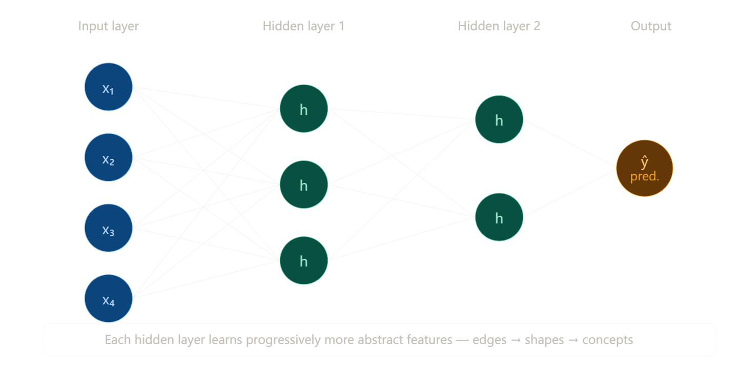
Stacking neurons into a network

A single neuron is limited. Real power comes from stacking layers. The input layer receives raw data, hidden layers learn intermediate representations, and the output layer produces a prediction.---

How does a network learn? (Backpropagation)

Learning is the process of adjusting weights to minimize error. It works in two passes:

Forward pass — data flows left to right, producing a prediction. Loss — we measure how wrong the prediction is (e.g., mean squared error or cross-entropy). Backward pass — the error is propagated backwards using the chain rule of calculus; each weight gets a gradient telling it which direction to move. Update — weights shift slightly in the direction that reduces error: w ← w − η · ∂L/∂w, where η (eta) is the learning rate.

Repeat this over thousands of examples and the network gradually gets better — this is called gradient descent.The ball rolls downhill toward the minimum loss. Try different learning rates — too large and it overshoots, too small and it’s painfully slow.

Transclude of gradient_descent_interactive

Activation functions

Without non-linear activations, stacking layers would do nothing beyond a single layer (all linear transformations compose into one). The three you’ll use most:

Function	Formula	Best for
ReLU	max(0, x)	Hidden layers — fast, avoids vanishing gradients
Sigmoid	1 / (1 + e⁻ˣ)	Binary classification output
Softmax	eˣⁱ / Σeˣʲ	Multi-class output (sums to 1)

What to learn next

Practical skills — implement a simple network in Python with PyTorch or TensorFlow.

Key concepts — overfitting and regularization (dropout, weight decay), batch normalization, optimizers beyond vanilla gradient descent (Adam, RMSProp), and loss functions for different tasks.

Neural Network-Tuned PID Controller for Servo Motor Position Control

1. Objective

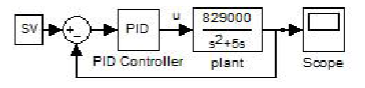
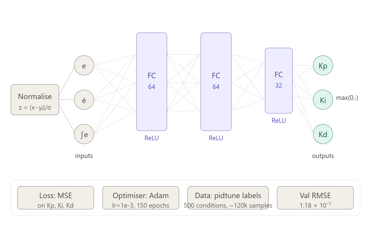
Design and implement a neural network that tunes the parameters of a PID controller in real time to control the position of a servo motor. The network receives the current error state of the closed-loop system as input and outputs the proportional, integral, and derivative gains (Kp, Ki, Kd) at each timestep. The entire workflow — data generation, training, and simulation — was carried out in MATLAB R2021a and Simulink.

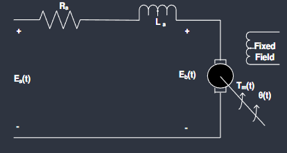
2. Plant Model

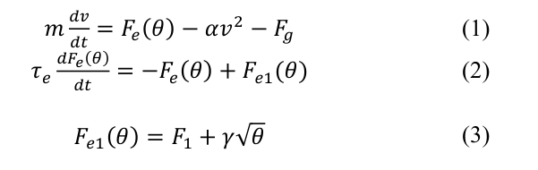
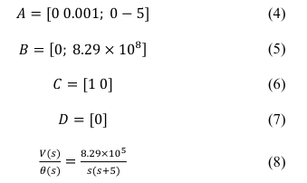
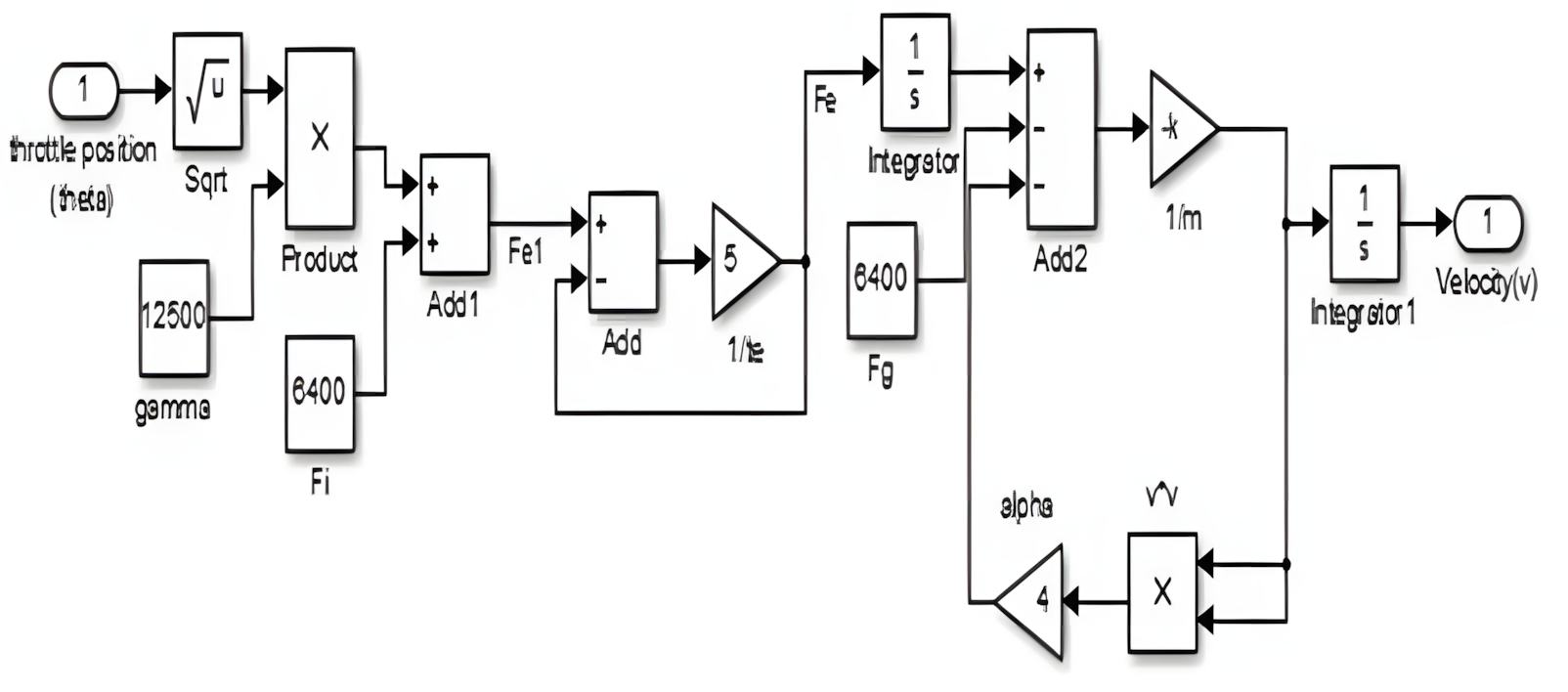
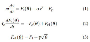
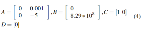
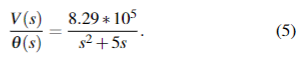
The servo motor was modelled as a second-order continuous-time transfer function:

G(s) = 8.29 × 10^5 / (s^2 + 5s)

This represents a DC motor driving a positional load, where:

The numerator gain of 8.29 × 10^5 reflects the combined motor torque constant and load scaling.
The denominator s^2 + 5s = s(s + 5) yields two open-loop poles: one at the origin (s = 0, the position integrator) and one at s = −5 (representing friction/damping).
The pole at the origin makes the plant Type 1, meaning it can track step inputs with zero steady-state error under proportional control, but also makes it sensitive to high gains.

In Simulink the plant was implemented as a Transfer Fcn block with numerator [829000] and denominator [1 5 0].

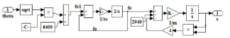
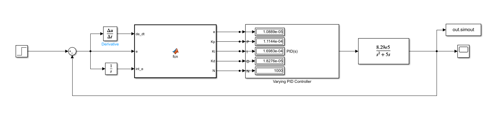
3. Control Architecture

The overall system is a neuro-adaptive PID loop. The neural network sits in parallel with the closed-loop, observing the error state and adjusting the PID gains in real time. The structure is:

Setpoint ──→ [Sum] ──→ [State signals] ──→ [Neural network] ──→ [PID Controller] ──→ [Plant G(s)] ──→ Output
                ↑                                                                                         │
                └─────────────────────────────────── feedback ───────────────────────────────────────────┘

The three state signals fed to the network are:

e(t) — current tracking error
de/dt — rate of change of error (computed via a discrete-time derivative block)
∫e dt — accumulated error (computed via an integrator block)

The network outputs Kp, Ki, Kd which are wired directly into the external gain input ports of the Simulink PID Controller block (variable gains mode). A filter coefficient N = 1000 was set on the derivative term of the PID block to suppress high-frequency noise.

4. Neural Network Design

4.1 Architecture

A feedforward fully-connected regression network was used:

Layer	Type	Neurons	Activation
Input	Feature input	3	—
fc1	Fully connected	64	ReLU
fc2	Fully connected	64	ReLU
fc3	Fully connected	32	ReLU
Output	Fully connected	3	Linear

Input: [e, de/dt, ∫e] — Output: [Kp, Ki, Kd]

The output layer uses a linear activation (no softmax or ReLU) so that the network can produce continuous-valued gains without artificial lower bounds beyond the max(0, ·) clamp applied post-prediction.

4.2 Approach — Supervised Imitation of pidtune

The network was trained using supervised learning. The training objective was to learn a mapping from error state to PID gains, where the target gains were generated by MATLAB’s pidtune() function across a sweep of operating conditions. This approach avoids the need for a reward function and is significantly simpler to implement than reinforcement learning for an initial prototype.

At inference time in Simulink, the network acts as an online gain scheduler — it continuously reads the error state and adjusts the PID gains based on the patterns it learned during training.

5. Training Data Generation

5.1 Procedure

500 operating conditions were simulated. For each condition:

The plant gain was randomly perturbed by ±10% around the nominal value (8.29 × 10^5) to build robustness to real-world parameter variation.
pidtune() was called on the perturbed plant to obtain optimal Kp, Ki, Kd for that condition.
A closed-loop step response was simulated using Euler integration over 2 seconds at dt = 0.005 s.
At each timestep, the state vector [e, de/dt, ∫e] was recorded as a feature row, and the gains from step 2 were recorded as the corresponding label row.

Conditions where pidtune() produced gains outside a physically sensible range were rejected (see Section 5.2). The accepted conditions produced approximately 120,000 training samples in total.

5.2 Iterations on pidtune Options

Two versions of the training script were developed:

Version 1 (create_pid_deep_net_v1.m)

opts = pidtuneOptions('CrossoverFrequency', 30, 'PhaseMargin', 60);

300 conditions, no gain clamping. Training converged but the network produced gains approximately 7–13× higher than what pidtune would give on the nominal plant. Specifically:

Gain	pidtune (nominal)	Network output	Ratio
Kp	6.36 × 10^-5	4.43 × 10^-4	~7×
Ki	8.13 × 10^-5	1.09 × 10^-3	~13×
Kd	1.11 × 10^-5	3.53 × 10^-5	~3×

The result was significant overshoot (~25%) and initial oscillation. Root cause: the gain variation loop during data generation occasionally produced high-gain conditions that were included in training without filtering, skewing the learned mapping upward. Additionally, a phase margin of 60° is permissive enough that pidtune produces moderately aggressive gains across conditions.

Version 2 (create_pid_deep_net_v2.m)

opts = pidtuneOptions('CrossoverFrequency', 15, 'PhaseMargin', 75);
KP_MAX = 2e-4;  KI_MAX = 2e-4;  KD_MAX = 5e-5;

500 conditions with hard rejection of any sample outside the clamped gain ranges. This filters out the outlier high-gain training examples. The lower crossover frequency and higher phase margin push pidtune toward more conservative, better-damped gains across all conditions. The dataset after rejection was used for final training.

6. Input Normalisation

Before training, all three input features were standardised to zero mean and unit standard deviation:

x_norm = (x - mean(x)) / std(x)

The normalisation statistics (norm_stats.mean, norm_stats.std) were saved alongside the trained network weights and applied identically inside the Simulink MATLAB Function block at inference time. Omitting this step would cause the network to receive out-of-distribution inputs at runtime.

7. Training Configuration

Parameter	Value
Optimiser	Adam
Initial learning rate	1 × 10^-3
Learning rate schedule	Piecewise (drop by 0.3× every 40 epochs)
Max epochs	150
Mini-batch size	256
Train/validation split	85% / 15%
Validation patience	20 checks
Hardware	Single CPU

Training was run using trainNetwork from the Deep Learning Toolbox. The training progress plot (09-Apr-2026 21:54:14) shows rapid loss reduction in the first 500 iterations, with the curve flattening and meeting the validation criterion at epoch 11 of 150 (7,100 iterations, elapsed time 4 min 49 sec).

Final validation RMSE: 1.1789 × 10^-5

Training stopped early due to the validation patience criterion — the validation loss had plateaued and further training was not improving generalisation.

Neuro-PID Training Script — Overview

Training script

clc
clear
close all
 
s = tf('s');
G = 8.29e5 / (s^2 + 5*s);
 
opts_ref = pidtuneOptions('CrossoverFrequency',15,'PhaseMargin',75);
C_ref = pidtune(G,'PID',opts_ref) %gains référence
 
KP_MAX = 2e-4; %gains limites
KI_MAX = 2e-4;
KD_MAX = 5e-5;
 
N = 500; %Nbre d'itérations
dt = 0.005; 
t = 0:dt:2;
Ns = length(t);
 
setpoints = 0.1 + 4.9*rand(N,1); %références
 
X = [];
Y = [];
 
opts = pidtuneOptions('CrossoverFrequency',15,'PhaseMargin',75);
 
rej = 0;
 
for i = 1:N
 
    Gv = (8.29e5*(0.9+0.2*rand())) / (s^2+5*s); %modèle avec variation de gain
 
    try
        C = pidtune(Gv,'PID',opts);
    catch
        rej = rej + 1;
        continue
    end
 
    Kp = C.Kp; Ki = C.Ki; Kd = C.Kd;
 
    if Kp<=0 || Ki<0 || Kd<0 || ...
       Kp>KP_MAX || Ki>KI_MAX || Kd>KD_MAX
        rej = rej + 1;
        continue
    end %rejection de gains limites
 
    r = setpoints(i);
    x1 = 0; x2 = 0; %position et vitesse
    ie = 0; pe = 0; %intégrale de l'erreur et erreur précédente
 
    feat = zeros(Ns,3); %features (entrées)
    lab  = repmat([Kp Ki Kd],Ns,1); %labels (sorties)
 
    for k = 1:Ns %simulation du modèle
        e  = r - x1;  %erreur
        de = (e - pe)/dt;  %dérivée de l'erreur
        ie = ie + e*dt;  %intégrale de l'erreur
 
        u = Kp*e + Ki*ie + Kd*de; %loi de commande
 
        x1 = x1 + x2*dt;
        x2 = x2 + (-5*x2 + 8.29e5*u)*dt;
 
        feat(k,:) = [e de ie];
        pe = e;
    end
 
    X = [X; feat];
    Y = [Y; lab];
 
end
 
m = mean(X); %normalisation
s = std(X)+1e-8;
 
Xn = (X - m)./s;
 
norm_stats.mean = m;
norm_stats.std  = s;
 
n = size(Xn,1); %diviser les données (85%/15%)
idx = randperm(n);
nt = floor(0.85*n);
 
Xtr = Xn(idx(1:nt),:); %données d'entrainement
Ytr = Y(idx(1:nt),:);
 
Xv  = Xn(idx(nt+1:end),:); %données de validation
Yv  = Y(idx(nt+1:end),:);
 
layers = [
    featureInputLayer(3,'Normalization','none')
    fullyConnectedLayer(64)
    reluLayer
    fullyConnectedLayer(64)
    reluLayer
    fullyConnectedLayer(32)
    reluLayer
    fullyConnectedLayer(3)
    regressionLayer
]; %architecture du réseau
 
opts = trainingOptions('adam', ...
    'MaxEpochs',150, ...
    'MiniBatchSize',256, ...
    'InitialLearnRate',1e-3, ...
    'ValidationData',{Xv,Yv}, ...
    'ValidationFrequency',50, ...
    'Shuffle','every-epoch', ...
    'Plots','training-progress'); %options du réseau
 
net = trainNetwork(Xtr,Ytr,layers,opts); %entrainement du réseau
 
Yp = predict(net,Xv); %calcul des prédictions
 
for i=1:3
    rmse = sqrt(mean((Yp(:,i)-Yv(:,i)).^2)); %calcul de l'erreur du réseau
end
 
xt = ([1 0 0]-m)./s;
gt = predict(net,xt); %test de prédiction
 
save('neuro_pid_net.mat','net','norm_stats')
 
W1 = net.Layers(2).Weights; b1 = net.Layers(2).Bias; %poids et biais du réseau
W2 = net.Layers(4).Weights; b2 = net.Layers(4).Bias;
W3 = net.Layers(6).Weights; b3 = net.Layers(6).Bias;
W4 = net.Layers(8).Weights; b4 = net.Layers(8).Bias;
 
save('neuro_pid_weights.mat','W1','b1','W2','b2','W3','b3','W4','b4','norm_stats')

Objective

The goal of this program is to train a neural network that can estimate PID controller gains
(Kp, Ki, Kd) based on the current state of the system:

error $e$
derivative of error $\overset{e}{˙}$
integral of error $\int e$

Plant Model

The system being controlled is defined as: $G (s) = \frac{8.29 * 1 0 ^{5}}{s ^{2} + 5 s}$

Data Generation

Training data is generated by simulating multiple operating conditions:

Random setpoints
Plant gain variation to simulate uncertainty
For each condition, a PID controller is tuned using MATLAB’s pidtune()

The system is then simulated over time:

Position and velocity states are updated step-by-step
At each timestep, the following are recorded:
- Features: [e, de/dt, ∫e]
- Labels: [Kp, Ki, Kd]

Invalid or extreme PID gains are filtered out.

Data Preprocessing

The input features are normalized using:

Mean
Standard deviation

This improves neural network training performance.

Neural Network Model

A feedforward neural network is used for regression:

Input:

3 features (e, de/dt, ∫e)

Architecture:

Fully connected layers: 64 → 64 → 32 neurons
Activation: ReLU
Output: 3 values (Kp, Ki, Kd)

The network is trained using:

Optimizer: Adam
Loss function: Mean Squared Error (MSE)

Training and Validation

The dataset is split:

85% training
15% validation

Model performance is evaluated using RMSE between predicted and true gains.

Results

The trained network is tested on validation data:

Predicted gains are compared to true gains
Scatter plots visualize prediction accuracy
A test input is used to compare NN output vs pidtune() reference

Output

The script saves:

neuro_pid_net.mat → trained network + normalization data
neuro_pid_weights.mat → extracted weights for Simulink use

8. Simulink Compatibility Issue and Resolution

8.1 Problem

The initial MATLAB Function block implementation passed the trained SeriesNetwork object (net) as an input port to the block and called predict(net, features) using coder.extrinsic. This failed with:

“The training data set has N features but the input layer expects 3.”

This error arose from two separate issues:

Transpose orientation error — trainNetwork with featureInputLayer expects data in row-major format (samples × features). The original script transposed X_train and X_val to column-major, causing the dimension mismatch. Fixed by removing the ' transpose operators from the feature matrices while retaining them on the label matrices — then corrected further in v2 to remove all transposes consistently.
SeriesNetwork incompatibility with Simulink — MATLAB R2021a’s Simulink cannot resolve SeriesNetwork object methods at code generation time, even with coder.extrinsic. Passing a network object as a Simulink signal is not supported.

8.2 Solution — Manual Forward Pass

The network object was eliminated from Simulink entirely. A separate script (load_weights.m) extracted the raw weight matrices and bias vectors from each layer:

W1 = net.Layers(2).Weights;  b1 = net.Layers(2).Bias;
W2 = net.Layers(4).Weights;  b2 = net.Layers(4).Bias;
W3 = net.Layers(6).Weights;  b3 = net.Layers(6).Bias;
W4 = net.Layers(8).Weights;  b4 = net.Layers(8).Bias;
save('neuro_pid_weights.mat', 'W1','b1','W2','b2','W3','b3','W4','b4','norm_stats');

The MATLAB Function block was rewritten to perform the forward pass manually using only matrix arithmetic — no toolbox objects, no predict, no coder.extrinsic:

function [Kp, Ki, Kd] = fcn(e, de_dt, int_e)
    persistent W1 b1 W2 b2 W3 b3 W4 b4 feat_mean feat_std
    if isempty(W1)
        data = load('neuro_pid_weights.mat');
        W1 = data.W1;  b1 = data.b1;
        W2 = data.W2;  b2 = data.b2;
        W3 = data.W3;  b3 = data.b3;
        W4 = data.W4;  b4 = data.b4;
        feat_mean = data.norm_stats.mean;
        feat_std  = data.norm_stats.std;
    end
    x = ([e, de_dt, int_e] - feat_mean) ./ feat_std;
    x = x';
    x = max(0, W1*x + b1);
    x = max(0, W2*x + b2);
    x = max(0, W3*x + b3);
    x = W4*x + b4;
    Kp = max(0, x(1));
    Ki = max(0, x(2));
    Kd = max(0, x(3));
end

persistent variables ensure the weights are loaded from disk only once at simulation start, not at every timestep. This approach is fully compatible with Simulink in R2021a and has no external dependencies.

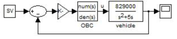
9. Simulink Model

The final model (neuro_pid_test.slx) consists of the following blocks:

Block	Configuration
Step	Step time = 0.1 s, Final value = 1.0
Sum	Signs: `+−`
Derivative	Discrete-time (Δu/Δt)
Integrator	`1/s`
MATLAB Function (`fcn`)	3 inputs (e, de_dt, int_e), 3 outputs (Kp, Ki, Kd)
PID Controller	Variable gains mode, external Kp/Ki/Kd/N ports
Constant (N)	N = 1000
Transfer Fcn	Num: `[829000]`, Den: `[1 5 0]`
Scope	Output position θ(t)
To Workspace (`out.simout`)	Logs output signal

The derivative block is the discrete-time variant (Δu/Δt) rather than the continuous Derivative block, which avoids the algebraic loop and impulse at t = 0 that the continuous block produces with a step input.

The N port of the PID block was initially set to 10, which produced visible oscillatory behaviour. Increasing N to 100 eliminated the oscillations, and the final value of N = 1000 was used in the submitted model.

10. Results

10.1 Step Response

Simulation duration: 3.0 seconds. Unit step setpoint applied at t = 0.

The stepinfo function returned the following performance metrics:

Metric	Value
Rise time	0.12 s
Peak time	0.39 s
Settling time	1.16 s
Overshoot	7.99%

The response rises quickly to the setpoint, reaches a peak of approximately 1.08 at t ≈ 0.39 s, then decays smoothly to steady state by t ≈ 1.16 s with no oscillation. There is no steady-state error.

10.2 Gain Values at Steady State

At the end of the simulation the network was outputting:

Gain	Value
Kp	1.1144 × 10^-4
Ki	1.6983 × 10^-4
Kd	1.8276 × 10^-5

These are in a comparable range to the pidtune reference gains (Kp = 6.36 × 10^-5, Ki = 8.13 × 10^-5, Kd = 1.11 × 10^-5) obtained for the nominal plant at 75° phase margin.

11. Issues Encountered and Resolutions

Issue	Cause	Resolution
`trainNetwork` dimension error (“N features but expects 3”)	X_train transposed to column-major (features × samples); `featureInputLayer` expects row-major	Removed transpose operators from X_train and X_val
SeriesNetwork incompatible with Simulink MATLAB Function	R2021a Simulink cannot resolve network object methods at simulation time	Extracted raw weight matrices; replaced `predict()` with manual matrix forward pass
Network outputting gains 7–13× too large	High-gain outlier conditions included in v1 training data; low phase margin (60°)	v2: added hard gain bounds, raised phase margin to 75°, lowered crossover to 15 rad/s
Oscillatory step response (initial)	PID filter coefficient N = 10 insufficient for derivative noise suppression	Increased N: 10 → 100 → 1000
Residual 7.99% overshoot	Network trained to imitate pidtune which itself permits overshoot at 75° phase margin	Identified as the ceiling of the current approach; motivates progression to FOPID

12. Scripts Summary

File	Purpose
`create_pid_deep_net_v1.m`	Initial training script — 300 conditions, CrossoverFreq=30, PhaseMargin=60, no gain clamping
`create_pid_deep_net_v2.m`	Revised training script — 500 conditions, CrossoverFreq=15, PhaseMargin=75, hard gain bounds
`load_weights.m`	Post-training utility — extracts W/b matrices from `neuro_pid_net.mat` into `neuro_pid_weights.mat`
`oldfn.m`	Deprecated MATLAB Function block implementations using `predict()` and `coder.extrinsic` (non-functional in R2021a Simulink)
`shallow_neuro_pid.m`	Exploratory script — attempted `fitnet` / `train` API as alternative to `trainNetwork`
`create_fitnet.m`	Auto-generated by MATLAB Neural Fitting App — `fitnet` with Levenberg-Marquardt, 10 hidden neurons

13. Next Step — Fractional Order PID

The residual 7.99% overshoot represents the performance ceiling of the current approach, because the network is fundamentally limited by its training targets: it can only be as good as what pidtune produces, and pidtune at 75° phase margin inherently permits some overshoot.

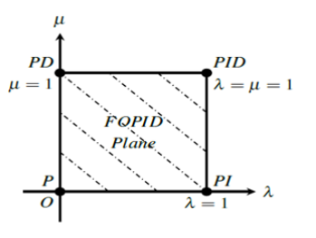
The proposed extension is to replace the integer-order PID with a Fractional Order PID (FOPID), which introduces two additional tunable parameters λ (fractional integration order) and μ (fractional differentiation order):

u(t) = Kp·e + Ki·D^{-λ}·e + Kd·D^{μ}·e,    λ,μ ∈ (0, 2)

This gives 5 parameters to tune instead of 3. The neural network will be extended to output all five: [Kp, Ki, Kd, λ, μ]. The fractional operators will be approximated in Simulink using Oustaloup filters. Training label generation will require replacing pidtune with an optimisation-based tuner (e.g. fmincon or particle swarm) since no direct equivalent of pidtune exists for FOPID.

Expected benefits for this plant: reduced overshoot (λ < 1 softens integral windup), faster settling (μ > 1 strengthens damping), and improved robustness to plant parameter variation.

Fractional PID

Estimation of fractional variables

Oustaloup Method

to estimate $s^{α}$ using the Oustaloup method:

we start by defining a frequency range $[ω_{l}, ω_{h}]$ and the number of cells $N$
we then generate the poles and zeros corresponding to the number of cells

ω_{z_{k}} = ω_{l} . (\frac{ω _{h}}{ω _{l}})^{\frac{k + N + 1 - α /2}{2 N + 1}}, ω_{p_{k}} = ω_{l} . (\frac{ω _{h}}{ω _{l}})^{\frac{k + N + 1 + α /2}{2 N + 1}}

we then calculate a generalized derivator

D_{g e n} (s) = (\frac{s}{ω _{c}})^{α}

we then approximate this generalized derivator with a real order transfer function

D_{N} (s) = (\frac{ω _{c}}{ω _{h}})^{α} k = - N \prod N \frac{1 + \frac{s}{z _{k}}}{1 + \frac{s}{p _{k}}}

D (s) = N \to \infty lim D_{N} (s)

we then adjust the gain

K = ω_{h}^{α}

we then calculate the the final transfer function that estimates $s^{α}$

H_{o u s t a l o u p} (s) = ω_{h}^{α} k = - N \prod N \frac{1 + \frac{s}{z _{k}}}{1 + \frac{s}{p _{k}}}

we get a transfer function with an order corresponding with the number of poles/zeros chosen

RayaneKch

Explorer

Contrôleur PID réglé par réseau de neurones - PFE

Pre-Choice

Choice

Key points

References to check out

Previous works & understanding

Optimal Fractional Order PID Controller for Speed Control of Electric Vehicle (ACO)

File

Outline

Breakdown

Optimal Speed Control of Hybrid Electric Vehicles (LQR)

File

Outline

Breakdown

Robust adaptive speed control of uncertain hybrid electric vehicle (H∞​ Control)

File

Outline

Breakdown

Tuning of PID Controller for DC Servo Motor using Genetic Algorithm

File

Outline

Breakdown

Contrôleur PID d’ordre fractionnaire basé sur la fonction idéale de Bode

File

Outline

Breakdown

Mémoire Structure

Introduction Générale

Chapitre I : État de l’art sur la Commande PID

Chapitre II : Fondamentaux des Réseaux de Neurones Artificiels

Chapitre III : Modélisation du Système à Commander

Chapitre IV : Conception du PID Auto-réglé par Réseau de Neurones

Chapitre V : Simulation et Analyse des Résultats

Conclusion Générale et Perspectives

Neural Networks

What is a neuron?

Stacking neurons into a network

How does a network learn? (Backpropagation)

Activation functions

What to learn next

Neural Network-Tuned PID Controller for Servo Motor Position Control

1. Objective

2. Plant Model

3. Control Architecture

4. Neural Network Design

4.1 Architecture

4.2 Approach — Supervised Imitation of pidtune

5. Training Data Generation

5.1 Procedure

5.2 Iterations on pidtune Options

6. Input Normalisation

7. Training Configuration

Neuro-PID Training Script — Overview

Training script

Objective

Plant Model

Data Generation

Data Preprocessing

Neural Network Model

Training and Validation

Results

Output

8. Simulink Compatibility Issue and Resolution

8.1 Problem

8.2 Solution — Manual Forward Pass

9. Simulink Model

10. Results

10.1 Step Response

10.2 Gain Values at Steady State

11. Issues Encountered and Resolutions

12. Scripts Summary

13. Next Step — Fractional Order PID

Fractional PID

Estimation of fractional variables

Oustaloup Method

Mémoire

Graph View

Table of Contents

Robust adaptive speed control of uncertain hybrid electric vehicle ( $H_{\infty}$ Control)